Linear Regression using Gradient Descent algorithm

Introduction

This tutorial aims to introduce the concept of linear regression, which is one of the bases to create your own neural network. For this tutorial, I would use a NASA csv on the surface temperature of the Earth link. The goal is to define a line representing the best fit, for a data collection

Definition

Linear regression is a linear approach for modeling the relationship between a scalar dependent variable y and one or more explanatory variables (or independent variables) denoted X.

GISS Surface Temperature Analysis from NASA

For this tutorial, i will use plotly with is a conveniant way to create interactive plot.

from plotly import __version__
from plotly.offline import download_plotlyjs, init_notebook_mode, plot, iplot

init_notebook_mode(connected=True)

import plotly.plotly as py
import plotly.graph_objs as go
import plotly.figure_factory as FF

print (__version__) # requires version >= 1.9.0

2.2.1

For this algoritm, you will need to use matrix so we import numpy and pandas in order to do matrix operation

import numpy as np
import pandas as pd

We can start by importing our csv data

#Load dataset .csv
df = pd.read_csv('GLB.Ts+dSST.csv')

#Create an interacrtive plot with plotly
sample_data_table = FF.create_table(df.head())
iplot(sample_data_table, filename='sample-data-table')

Display all the data with plotly

traces = []
for month in df:
    #Add one trace by raw exept for the 'Year' raw
    if (month != 'Year'):
        traces.append(go.Scatter(
                      x = df['Year'], y = df[month],
                      name= month
                      ))
#Definining layout for ours traces
layout = go.Layout(
                  title='Global-mean monthly, seasonal, and annual means (1880-present)',
                  plot_bgcolor='rgb(230, 230,230)', 
                  showlegend=True
                  )

#Create the figure
fig = go.Figure(data=traces, layout=layout)

#Display the graph
iplot(fig, filename='GLB.Ts+dSST')

These curves represent the temperature anomalies from 1880 to present, i.e. deviations from the corresponding 1951-1980 means.

Linear regression error (formula)

Linear regression error (Implementation)

#Implementation of the linear regression error formula (just above)
def LinearRegressionError(b, m, values):
    error = 0
    for val in values:
        error += (val[1] - (m * val[0] + b)) ** 2
    return error / float(len(values))

Linear regression gradient (formula)

Linear regression gradient (Implementation)

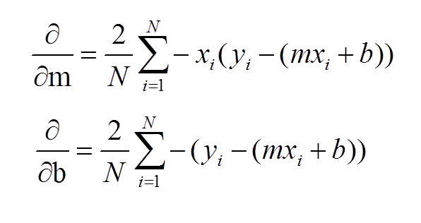
#Implementation of the linear regression gradiant formula (just above)
def step_gradient(current_b, current_m, values, learing_rate):
    gradient_b = 0
    gradient_m = 0
    n = len(values)
    for val in values:
        gradient_m += -(2 / n) * val[0] * (val[1] - (current_m * val[0] + current_b))
        gradient_b += -(2 / n) * (val[1] - (current_m * val[0] + current_b))
    new_b = current_b - (learing_rate * gradient_b)
    new_m = current_m - (learing_rate * gradient_m)
    return [new_b, new_m]

Create the run function

#iniatial_b = -20
#iniatial_m = -20
#number_iteration = 8000
#learning_rate = 0.0001

#Best fit line :
#Y = M * X + B

#define global B and M for drawing later
B = 0
M = 0

def run(initial_b, initial_m, number_iteration, learning_rate):
    b = initial_b
    m = initial_m
    values = []
    for i in range(len(df['Year'])):
        values.append([df['Year'][i] * 0.01, df['Jan'][i]])
    print("Starting gradient descent at b = {0}, m = {1}, error = {2}".format(initial_b, initial_m, LinearRegressionError(initial_b, initial_m, values)))
    #Start gradiant descent, update local m and b
    for i in range(number_iteration):
        [b, m] = step_gradient(b, m, values, learning_rate)
    print("After {0} iterations b = {1}, m = {2}, error = {3}".format(number_iteration, b, m, LinearRegressionError(b, m, values)))
    global B
    global M
    B = b
    M = m

if __name__ == '__main__':
    run(-20, -20, 8000, 0.0001)

Starting gradient descent at b = -20, m = -20, error = 167932.21884420287
After 8000 iterations b = -18.92211864597688, m = 0.9716309040346014, error = 0.050925591977459134

#Define dot traces
trace = go.Scatter(
    x = df['Year'], y = df['Jan'],
    name= 'Jan',
    mode='markers',
    marker=dict(
        color='rgba(255, 165, 196, 0.95)',
        line=dict(
            color='rgba(156, 165, 196, 1.0)',
            width=1,
        ),
            symbol='circle',
            size=10,
        )
    )
xTab = [1880, 2017]
#Y = M * X + B
yTab = [(M * xTab[0] * 0.01 + B), (M * xTab[1] * 0.01 + B)]

#Define best fit trace
trace1 = go.Scatter(
    x = xTab,
    y = yTab,
    name = 'Best fit'
)

#Define the layout
layout = go.Layout(
    title='January anomaly from 1880 to present',
    plot_bgcolor='rgb(230, 230,230)',
    showlegend=True
)

#Draw the final graph
fig = go.Figure(data=[trace, trace1], layout=layout)
iplot(fig, filename='dot_Jan')

Links

Youtube

• Siraj Raval

Web

• Matt Nedrich
• Introduction to Gradient Descent Algorithm
• Wikipedia - Linear regression
• Wikipedia - Gradient descent

Data

• GISS Surface Temperature Analysis - NASA